Continuous targets
ContinuousOverlapIndex is the regression counterpart to the discrete-label
estimator. It asks whether nearby feature prototypes contain compatible
empirical target distributions, then calibrates the observed disagreement
against shuffled target assignments.
from sklearn.preprocessing import MinMaxScaler
from overlapindex import ContinuousOverlapIndex

X = MinMaxScaler().fit_transform(X)

coi = ContinuousOverlapIndex(
    model_type="MiniBatchKMeans",
    kmeans_k=8,
    kmeans_kwargs={"random_state": 0},
    n_target_cells="auto",
    n_null_permutations=20,
    random_state=0,
).fit(X, y_regression)

print(coi.index)
print(coi.actual_loss_, coi.null_loss_)
The estimator is offline-first. MiniBatchKMeans, KMeans, and BallCover are
supported; partial_fit refits on the supplied batch and does not retain
continuous-target state across calls.
KMeans and MiniBatchKMeans also accept SciPy sparse feature matrices. Sparse inputs remain in CSR form through prototype fitting, adjacency scoring, and permutation-null refits; continuous targets remain dense numeric arrays.
random_state seeds target-cell construction, projection directions,
permutation sampling, and the selected feature backend. An explicit
random_state inside kmeans_kwargs or ballcover_kwargs takes precedence
for that backend.
The fitting pipeline
Scale the continuous target columns according to
target_scaling.Partition target space into pseudo-label cells.
Fit label-owned feature prototypes using those cells.
Build prototype adjacency in feature space.
Measure disagreement between empirical target distributions on adjacent prototypes.
Compare actual loss with a permutation-null loss and aggregate local prototype indices.
The support-weighted calibration follows
Thus 1.0 represents no observed harmful overlap, values between 0.0 and
1.0 represent partial separation, and 0.0 represents complete or
permutation-equivalent overlap. All reported local and aggregate values are
bounded to [0, 1]. A loss_ratio_ above 1.0 identifies worse-than-null
disagreement while the index remains at the lower endpoint.
Target cells and distances
Target shape |
|
|
|---|---|---|
Univariate |
Quantile cells |
1D Wasserstein distance |
Multivariate |
KMeans cells |
Sliced Wasserstein distance |
n_target_cells="auto" resolves to a sample-size-dependent value between 8
and 64, capped by the number of samples. Too few cells can hide target
structure; too many may leave cells and their feature prototypes poorly
supported. For multivariate targets, set random_state and optionally
target_cover_kwargs for reproducible KMeans cells.
target_scaling="standard" is the default. The alternatives are "none",
"minmax", and "robust". Scaling is particularly important when
multivariate target columns use different units.
Feature adjacency
The default adjacency_mode="soft_topk" spreads each sample’s competitor mass
over up to top_k nearby non-own prototypes. feature_temperature controls
the concentration: smaller values approach a single dominant competitor.
Use adjacency_mode="hard_top1" for strict single-competitor scoring or
backwards comparisons. Keep adjacency settings constant when comparing
representations.
Continuous behavior gallery
The main synthetic gallery follows three genuinely continuous regression
problems: a smooth latent signal with increasing observation fidelity, a
folded latent trajectory that is progressively unfolded in feature space, and
a continuous covariate that is gradually recovered. It uses eight target
cells, rather than reducing each problem to a high-versus-low split, and
strict nearest-competitor adjacency so the ideal target-ordered endpoints
approach the 1.0 anchor.
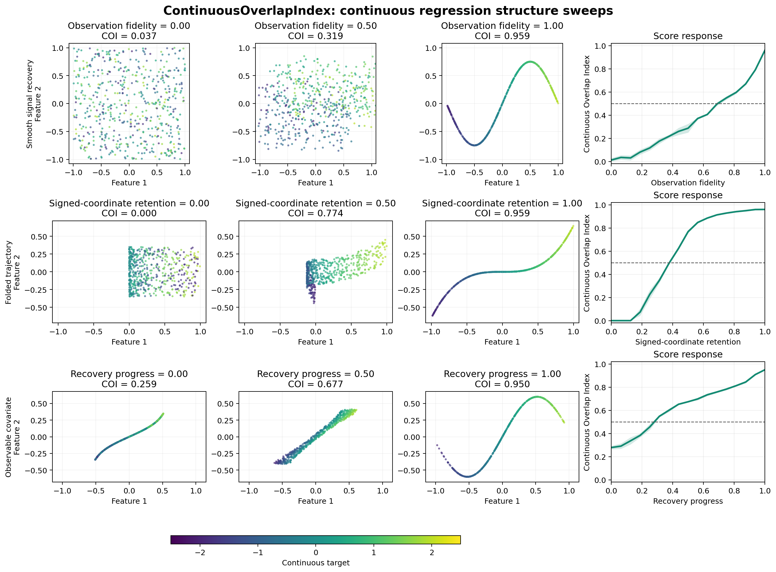
Regenerate it from the repository root with:
poetry run python examples/visualize_continuous_overlap_sweeps.py
An additional gallery shows a heteroscedastic target field becoming cleaner and a multivariate oscillator target observed with increasing fidelity:
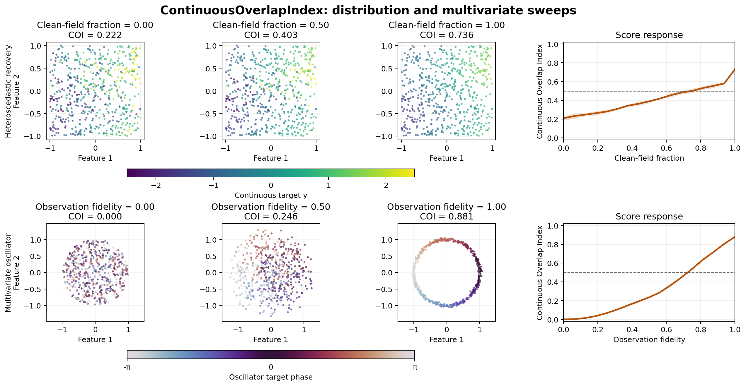
poetry run python examples/visualize_continuous_overlap_additional_sweeps.py
The example scripts use six refit permutations per score to keep the complete
sweeps practical to reproduce. Increase n_null_permutations when adapting
them for final quantitative reporting.
Permutation nulls
null_mode="refit_permutation"rebuilds target cells and feature prototypes for every shuffle. It provides the strongest null semantics and is the best choice for final reporting when affordable.null_mode="fixed_structure_permutation"keeps fitted prototype geometry and shuffles targets across it. It is substantially faster but approximate.null_mode="auto"uses the refit mode whenn_samples * n_null_permutations < auto_null_work_threshold, otherwise the fixed-structure mode. The default threshold is100_000.
Inspect null_mode_ after fitting to see which mode actually ran. Increase
n_null_permutations for a more stable null estimate, trading off runtime.
null_loss_samples_ contains the individual draws.
Aggregation and diagnostics
aggregation="support_weighted" is the default, so index calibrates the
support-weighted prototype loss. With aggregation="macro", index is the
unweighted mean of the bounded prototype indices and macro_index_ contains
the same value. The weighted_index property is always available regardless
of the selected aggregation.
Useful fitted attributes include:
actual_loss_,null_loss_, andloss_ratio_for calibration.prototype_index_,prototype_loss_, andprototype_support_for local diagnosis.prototype_target_values_,prototype_target_mean_, andprototype_target_cov_for target summaries.prototype_adjacency_andprototype_adjacency_normalized_for the feature neighborhood graph.target_cell_ids_,target_cover_, andtarget_distance_for resolved target-space choices.
The prototype target attributes retain empirical target measures rather than reducing every prototype to only a mean or variance. This is what allows the configured Wasserstein distance to compare richer local target distributions.
Continuous and discrete scores use related interpretation anchors but different calibrations. Do not directly compare an OI from one estimator with a COI from the other.
Calibration migration
The continuous calibration changed in the 0.1.3 alpha series. At the
loss-ratio level, the new pre-bound calibration equals
2 * legacy_score - 1, after which values are bounded to [0, 1]. Historical
and recalibrated COI values should not be compared directly.